

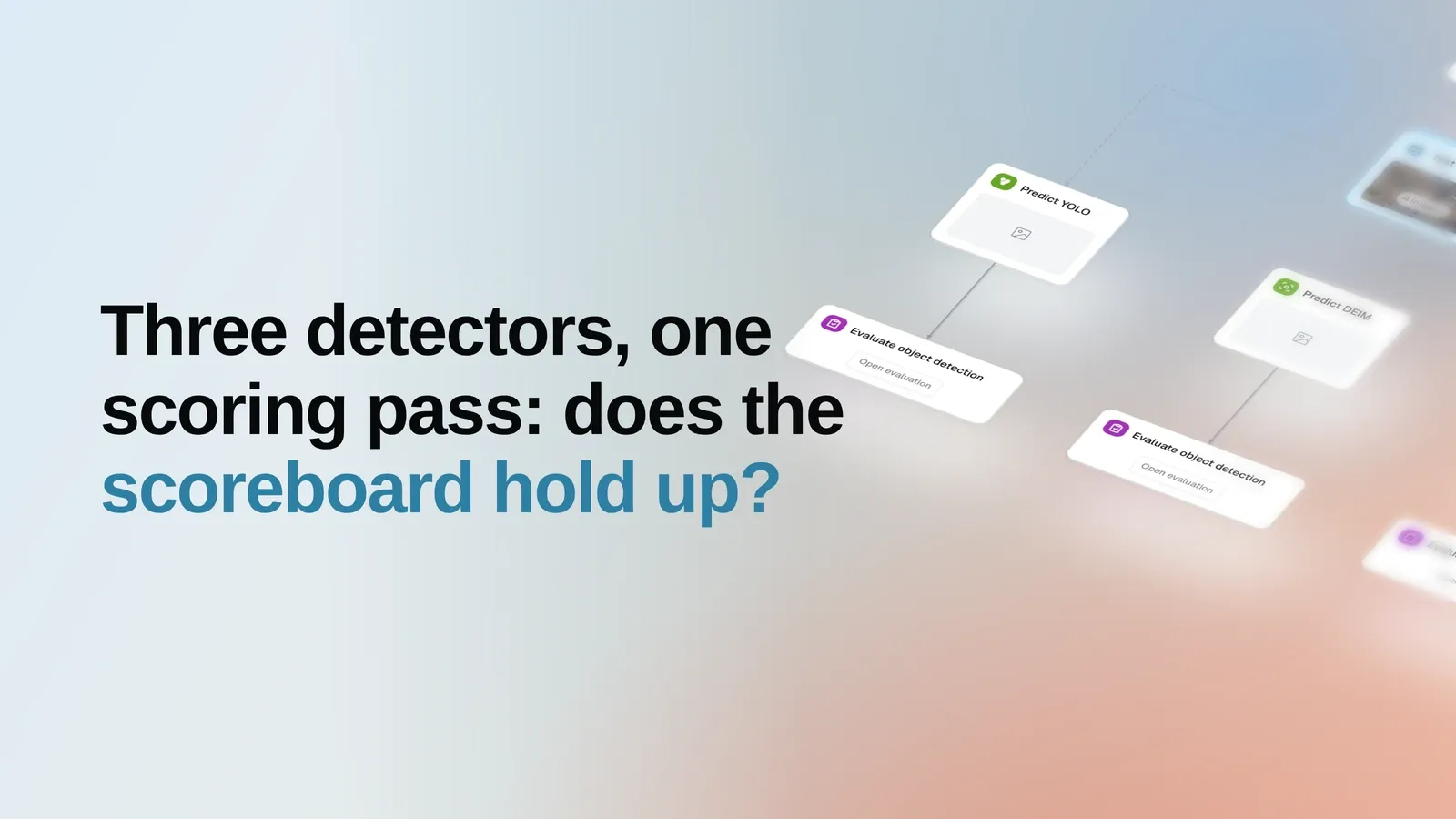
The thing under test here is the scoreboard, not the model
Every model decision downstream rests on one number that somebody’s evaluation code printed. Swap the matching rule, the confidence cut-off, or the reference set, and the same predictions gain or lose several points without a single weight changing. So the honest first question about an evaluation setup is not which model won — it is whether the scoring behaves the way a reader would expect on material they can check for themselves.
That question is nearly impossible to answer on private data, because there is nothing to hold the result against. It is easy to answer on a public reference the field already knows: take several unrelated, ready-made models, push them through one scoring pass against one reference, and see whether the resulting spread is sane.
What differs between the three columns is the model, and nothing else
Three detectors from three unrelated families are taken exactly as their authors published them:
ecdet_s (EdgeCrafter), yolov8s (YOLOv8s), and deimv2_hgnetv2_n (DEIM). No fine-tuning, no
per-model threshold tuning, no re-labelling. Each predicts on the same 5,000 images, and each result
is scored by the same evaluation step against the same ground truth, at the same IoU threshold of
0.50 for threshold-dependent views and the same budget of 100 detections per image.
The run is deliberately short — import the reference set with its labels, predict three times, score three times — because a longer one would put more of its own machinery between the models and the number. Each of those stages is an ordinary step, reused unchanged from the same building blocks that score a team’s own private data. That is what makes this a rehearsal rather than a demo: the scoring pass that produced the table below is the scoring pass a team would point at their own held-out set tomorrow.
Why COCO val2017 is a fair place to ask
The reference is the standard COCO validation set: 5,000 images spanning 80 everyday classes and carrying 36,334 ground-truth objects. It was neither collected nor curated for this run, and it is the set all three model families were benchmarked on by their own authors — which is the point. A reader can hold this run against their own knowledge of the dataset instead of taking a report’s word for it.
It is also a deliberately unkind test. The class distribution is wildly skewed: person carries
10,777 ground-truth objects, toaster carries 9. Many objects are small, thin, or heavily occluded,
and no model here has seen a fine-tuning pass on this data. A scoring setup that flattered models
would show it on material this varied.
Three models, one scoreboard
Read across the row rather than down the column. The interesting thing is not that one model leads, but that the ordering is the same whichever companion metric you look at, and that every value lands in the range its family is known for.
| Model | Checkpoint | mAP | AP50 | AP75 | Precision | Recall | F1 | Mean IoU | Class acc. | Calibration | Operating point |
|---|---|---|---|---|---|---|---|---|---|---|---|
| EdgeCrafter | ecdet_s | 50.9% | 68.6% | 54.7% | 63.2% | 47.3% | 53.4% | 87.1% | 97.9% | 95.5% | 0.52 |
| YOLOv8s | yolov8s | 43.9% | 60.0% | 47.4% | 58.2% | 42.0% | 48.0% | 86.9% | 96.7% | 99.5% | 0.38 |
| DEIM | deimv2_hgnetv2_n | 42.4% | 59.5% | 45.5% | 56.5% | 39.9% | 45.9% | 85.6% | 96.9% | 94.1% | 0.49 |
EdgeCrafter leads at 50.9% mAP, ahead of YOLOv8s at 43.9% and DEIM at 42.4%. The lead is not an artefact of one threshold: it holds at the permissive matching criterion (68.6% AP50 against 60.0% and 59.5%) and at the strict one alike, and F1 orders the three the same way. A scoring setup with a bias baked into one particular matching rule would not produce a consistent ordering across all four.
The drop between the loose and strict criteria is worth a second look for its own sake. Each model loses roughly a fifth of its AP50 when the overlap requirement tightens to 0.75 — a spread of 12.6 to 14.0 points. That is the ordinary signature of box localization on cluttered scenes, not something specific to one architecture, and seeing all three lose about the same share is itself evidence that the strict criterion is being applied evenly.
The arithmetic underneath the scoreboard adds up
A metric table is only as trustworthy as the counting that produced it, so the first thing worth checking is not the ranking but the bookkeeping. Summed across the 80 classes, true positives plus false negatives come to exactly 36,334 for every one of the three models — the full ground-truth count, not a per-model subset of it. Nothing was skipped, double-counted, or scored against a different reference.
The shape of the errors is the same for all three, and it is the shape this data should produce: false negatives outnumber false positives by roughly three to one in every case. On a set with this many small and occluded objects, detectors miss far more than they invent — and the ordering of the missed-object counts follows the ordering of the scoreboard, as it should.
One number does not follow that pattern, and it is instructive. Before the 100-detection budget is applied, the three models emit very different volumes of raw boxes: about 1.50 million for DEIM, 1.50 million for EdgeCrafter, and 559 thousand for YOLOv8s — a 2.7x spread. The model that produced the most boxes is also the model that scored lowest. Volume is not what the scoring pass rewards, which is exactly what a reader should want to confirm before trusting the pass on their own data.
The lead is not an averaging artefact
An aggregate metric can hide almost anything. A model can win on mAP by dominating a handful of frequent classes while losing most of the others, and the single number will not say so. Here it does not happen: EdgeCrafter has the highest AP50 in 79 of the 80 classes.
Two things are visible at once. The gap between models is real but modest; the gap between classes
is enormous. Large, distinctive animals and vehicles score in the nineties for every model, while
book, apple, backpack, handbag, and knife sit in the twenties and thirties for all three.
Whatever separates these architectures matters far less than whether the objects a team cares about
are big and distinctive or small, thin, and cluttered — which is the argument for running an
evaluation on your own classes rather than reading a headline number off a public one.
The single class where the ordering flips is toaster, where YOLOv8s reaches 82.3% AP50 against
EdgeCrafter’s 63.4%. That class has 9 ground-truth objects in the entire reference set. A couple of
detections move it by tens of points, so it is noise rather than an architectural finding — and the
weakest class in the set, hair drier, has 11. Both are worth naming precisely so they are not
mistaken for evidence.
Where the rankings stop agreeing with each other
Quality is not the only axis a report measures, and the other axes do not obediently reproduce the mAP ordering.
Calibration — how well a model’s confidence scores match its observed correctness — puts YOLOv8s first at 99.5%, ahead of EdgeCrafter at 95.5% and DEIM at 94.1%, inverting the quality ranking for the leader. For anyone who plans to threshold on confidence, act on a score, or route low-confidence predictions to review, that is a more consequential property than a few points of mAP. Box tightness tells a third story: mean IoU on matched boxes is within 1.5 points across all three models (87.1%, 86.9%, 85.6%), and classification accuracy on correctly localized boxes is within 1.2 points (97.9%, 96.7%, 96.9%). Neither labelling nor box precision is what separates these models; finding the objects at all is.
The operating point deserves the same care. Precision, Recall, and F1 in the table are computed after each model’s own automatically selected confidence threshold — 0.52, 0.38, and 0.49 respectively — so those three columns compare models at three different cut-offs, each chosen to suit that model. mAP, AP50, and AP75 are free of that choice. When a comparison has to be airtight, the threshold-free metrics are the ones to quote.
What this run does not tell you
It does not compare its numbers against the figures the model authors published, because nothing in the run fetches or verifies those figures. Treat the table as three models measured the same way here, not as a verdict on anyone’s published claim.
It measures no speed, latency, memory, or cost. A detector that leads on mAP may be the wrong choice on an edge device, and this run contains no evidence either way.
It also contains no per-image visual comparison, and the reason is worth stating rather than hiding. All three prediction steps ran at a 0.001 confidence threshold, so the stored predictions are the full un-thresholded detection dump — hundreds of boxes per image. That is the correct input for computing average precision and the wrong thing to put in front of a reader as an illustration. Per-image inspection belongs in the live example, where the confidence overlay can be adjusted, not in a static figure that would misrepresent what any of these models actually outputs.
And nothing here is fine-tuned. These are three published checkpoints on a set none of them was adapted to, which is the point of the exercise and also its limit.
What becomes repeatable
The reusable part is the shape, not the dataset. Point the same three stages at a private held-out set and the output is the same scoreboard on data that actually matters to the team: same matching rule, same companion metrics, same per-class breakdown, same outcome counts to check the arithmetic against.
That is why the public reference is worth the compute. It is where the machinery can be audited in the open — where a reader can confirm that the counts reconcile, that the ordering survives four different metrics, that raw prediction volume buys nothing, and that tiny classes are visible as tiny — before anyone has to trust the same machinery on data nobody else can see.